
Tutorial 2: Helmholtz Equation in 2D
In our second tutorial we consider a two dimensional example, a Helmholtz Equation in 2D. To be more precise:
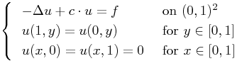
We calculate on the two-dimensional domain [0,1] x [0,1] with
-
periodic boundary conditions in the first dimension,
-
homogeneous Dirichlet boundary conditions in the second dimension,
i.e. we have
Again the solution is obtained using a uniform Wavelet-Galerkin method with a diagonal scaling preconditioner.
*
* This example calculates a Helmholtz problem on the two-dimensional domain [0,1]
* with periodic boundary conditions in the first dimension and Dirichlet conditions
* in the second dimension, i.e.
* - u_xx + c * u = f on (0,1)^2 ,
* u(1,y) = u(0,y) for y in [0,1],
* u(x,0) = u(x,1) = 0 for x in [0,1]
* The solution is obtained using a uniform Wavelet-Galerkin method with a
* diagonal scaling preconditioner.
*/
The complete example code in snippets:
#include <fstream>
#include <lawa/lawa.h>
using namespace std;
using namespace lawa;
Typedefs for Flens data types:
typedef flens::GeMatrix<flens::FullStorage<T, cxxblas::ColMajor> > FullColMatrixT;
typedef flens::SparseGeMatrix<flens::CRS<T,flens::CRS_General> > SparseMatrixT;
typedef flens::DiagonalMatrix<T> DiagonalMatrixT;
typedef flens::DenseVector<flens::Array<T> > DenseVectorT;
Typedefs for problem components:
Periodic Basis using CDF construction
Interval Basis using Dijkema construction
TensorBasis: uniform (= full) basis
typedef Basis<T, Primal, Interval, Dijkema> PrimalBasis_y;
typedef TensorBasis2D<Uniform, PrimalBasis_x, PrimalBasis_y> Basis2D;
HelmholtzOperator in 2D, i.e. for 
Preconditioner: diagonal scaling with norm of operator
Right Hand Side (RHS): basic 2D class for rhs integrals of the form  , with
 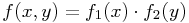 , i.e. the RHS is separable.
typedef SumOfTwoRHSIntegrals<T, Index2D, RHS2D, RHS2D> SumOf2RHS;
The constant 'c' in the Helmholtz equation.
The solution u is given as 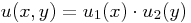 .
.
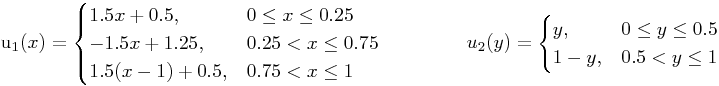
Right Hand Side for Laplace Operator and separable u (as given):

which will be represented as f_rhs_x * u1 + u2 * f_rhs_y.
{
if(x <= 0.25){
return 1.5*x + 0.5;
}
if(x <= 0.75){
return -1.5*x + 1.25;
}
return 1.5*(x-1.) + 0.5;
}
T u2(T y)
{
if(y <= 0.5){
return y;
}
return -y + 1;
}
T f_rhs_x(T x)
{
return 0.5 * c * u1(x);
}
T f_rhs_y(T y)
{
return 0.5 * c * u2(y);
}
T sol(T x, T y)
{
return u1(x) * u2(y);
}
T dx_sol(T x, T y)
{
if(x <= 0.25){
return 1.5 * u2(y);
}
if(x <= 0.75){
return -1.5 * u2(y);
}
return 1.5 * u2(y);
}
T dy_sol(T x, T y)
{
if(y <= 0.5){
return u1(x);
}
return -u1(x);
}
again we provide a function that writes the results into a file for later visualization.
printUandCalcError(const DenseVectorT u, const Basis2D& basis, const int J_x, const int J_y,
const char* filename, const double deltaX=0.01, const double deltaY=0.01)
{
T L2error = 0.;
T H1error = 0.;
ofstream file(filename);
for(double x = 0.; x <= 1.; x += deltaX){
for(double y = 0; y <= 1.; y += deltaY){
T u_approx = evaluate(basis, J_x, J_y, u, x, y, 0, 0);
T dx_u_approx = evaluate(basis, J_x, J_y, u, x, y, 1, 0);
T dy_u_approx = evaluate(basis, J_x, J_y, u, x, y, 0, 1);
file << x << " " << y << " " << u_approx << " " << sol(x,y) << " "
<< dx_u_approx << " " << dy_u_approx << endl;
T factor = deltaX * deltaY;
if((x == 0) || (x == 1.)){
factor *= 0.5;
}
if((y == 0) || (y == 1.)){
factor *= 0.5;
}
L2error += factor * (u_approx - sol(x, y)) * (u_approx - sol(x,y));
H1error += factor * (dx_u_approx - dx_sol(x,y))*(dx_u_approx - dx_sol(x,y))
+ factor * (dy_u_approx - dy_sol(x,y))*(dy_u_approx - dy_sol(x,y));
}
}
file.close();
H1error += L2error;
L2error = sqrt(L2error);
H1error = sqrt(H1error);
DenseVectorT error(2);
error = L2error, H1error;
return error;
}
First we check our arguments ...
{
/* PARAMETERS: */
if(argc != 7){
cerr << "Usage: " << argv[0] << " d d_ j0_x J_x j0_y J_y" << endl;
exit(-1);
}
... order of wavelets,
int d_ = atoi(argv[2]);
... minimal levels
int j0_y = atoi(argv[5]);
... maximal levels.
int J_y = atoi(argv[6]);
Basis initialization, setting Dirichlet boundary conditions in the second dimension
PrimalBasis_y b2(d, d_, j0_y);
b2.enforceBoundaryCondition<DirichletBC>();
Basis2D basis2d(b1, b2);
cout << "Cardinality of basis: " << basis2d.dim(J_x, J_y) << endl;
Operator initialization
DiagonalPrec p(a);
Right Hand Side:
Singular Supports in both dimensions
DenseVectorT sing_support_y(3);
sing_support_x = 0., 0.25, 0.75, 1.;
sing_support_y = 0., 0.5, 1.;
Forcing Functions
SeparableFunction2D<T> F2(u1, sing_support_x, f_rhs_y, sing_support_y);
Peaks: points and corresponding coefficients
(heights of jumps in derivatives)
FullColMatrixT deltas_y(1, 2);
FullColMatrixT nodeltas;
deltas_x = 0.25, 3,
0.75,-3;
deltas_y = 0.5, 2;
RHS2D rhs1(basis2d, F1, deltas_x, nodeltas, 2);
RHS2D rhs2(basis2d, F2, nodeltas, deltas_y, 2);
SumOf2RHS F(rhs1, rhs2);
Assemble equations system
SparseMatrixT A = assembler.assembleStiffnessMatrix(a, J_x, J_y);
DenseVectorT f = assembler.assembleRHS(F, J_x, J_y);
DiagonalMatrixT P = assembler.assemblePreconditioner(p, J_x, J_y);
Solve system
cout << pcg(P, A, u, f) << " pcg iterations" << endl;
Generate output for gnuplot visualization
return 0;
}